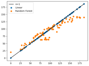
You should always try to use linear regression first when you are faced with an unknown data source for regression analysis, the main and simple reason behind this is:
Linear Regression creates a stable and accurate model, unlikely to fail miserably with erratic data.
If you are able to model the data correctly to fit a linear model, it is very likely that you have derived the true equation to solve the problem. Lets see an example with a very basic example with a very linear equation:
Y = x1+x2
from sklearn.linear_model import LinearRegression
from sklearn.ensemble import RandomForestRegressor
from sklearn.model_selection import train_test_split
import numpy as np
import matplotlib.pyplot as plt

# generating data
x1 = np.random.randint(100,size=100)
x2 = np.random.randint(100,size=100)
X = np.stack((x1,x2),axis=1)

# purely linear equation
y = x1+x2

# splitting data
X_train, X_test, y_train, y_test = train_test_split(X,y,test_size=0.8)

# linear regression
linearRegressor = LinearRegression()
linearRegressor.fit(X_train,y_train)
y_pred_linear = linearRegressor.predict(X_test)
print(linearRegressor.intercept_)  # prints near zero
print(linearRegressor.coef_)  # prints [1,1]

# random forest regression
randomForestRegressor = RandomForestRegressor(max_depth=100,n_estimators=100)
randomForestRegressor.fit(X_train,y_train)
y_pred_randomForest = randomForestRegressor.predict(X_test)

# plotting
plt.scatter(y_test,y_pred_linear,label='Linear')
plt.scatter(y_test,y_pred_randomForest,label='Random Forest')
plt.plot([np.min(y_test),np.max(y_test)],[np.min(y_test),np.max(y_test)],'k-',label='n=1')
plt.legend()
plt.show()
The results are shown below for degree of fit, additionally from printing the linear regression intercept and slope we can see that it derived the following equation:
Y = 1*x1+1*x2+0
Which is spot on.

